Part 0

1.What is Machine Learning?

Tom Mitchell in his book Machine Learning provides a definition in the opening line of the preface:

A computer program is said to learn from experience E with respect to some class of tasks T and performance measure P, if its performance at tasks in T, as measured by P, improves with experience E.

where,

T := The goal of the algorithm(prediction/classification/cluster).

P := The cost function of the algorithm.

E := The process of the algorithm.

Therefore, based on the definition above, I summarize five questions that we should ask to know about an algorithm and top 20 most popular machine learning algorithms. (BIG 5 $\times$ TOP 20)

BIG 5 QUESTIONS

1. What are the basic concepts/ What problem does it solve?

2. What are the assumptions?

3. What is the process of the algorithm?

4. What is the cost function?

5. What are the advantages and disadvantages?

TOP 20 ALGORITHMS

1. Linear Regression

2. Regression with Lasso

3. Regression with Ridge

4. Stepwise Regression

5. Logistic Regression

6. Naive Bayes

7. LDA (Linear Discriminant Analysis)

8. QDA (Quadratic Discriminant Analysis)

9. KNN (K-Nearest Neighbor)

10. Decision Tree

11. Random Forest

12. Boosting

13. Neural Network

14. K-means Clustering

15. SVM (Support Vector Machine)

16. PCA (Principal Component Analysis)

17. Bias-Variance Trade-off

18. Learning Curves

19. Anomaly Detection

20. Gradient Descent

Part I: TOP 20 $\times$ BIG 5

1. Linear Regression

1.1 What are the basic concepts/ What problem does it solve?

Basic concepts: A linear approach to model the relationship between continuous variables. ‘$X$’s are the predictors( or explanatory, or independent variables). ‘$Y$’ is the outcome( or response, or dependent variable). \
Model: $\hat{Y}= \theta X+ \epsilon$

1.2 What are the assumptions?

• The mean function is linear
• The variance function is constant
• Residuals are statistically independent, normally distributed with uniform variance
• The error term $\epsilon$ is assumed to be normally distributed with a mean of 0 and constant variance $\sigma^2$ at every value of $X$ (Homoscedastic)
• The error terms are assumed to be independent, that is $\epsilon \sim N(0,\sigma^2)$

1.3 What is the process of the algorithm?

We want to find the best fit line: $$ \hat{y_i}= \theta_0 + \theta_1 x_i $$

Usually, we achieve this by using least squares estimation, which finds the values of $\theta_0$ and $\theta_1$ that minimize the sum of the squared predicted errors: $$ \sum_{i=1}^n (y_i- \hat{y_i})^2 $$

thus we have, $$\theta_1= \frac {\sum_{i=1}^n (x_i-\bar{x}) (y_i-\bar{y})} {\sum_{i=1}^n (x_i−\bar{x})^2} $$

and $$\theta_0= \bar{y} - \theta_1 \bar{x}$$

1.4 What is the cost function?

$$J(\theta)= \frac{1}{n} \sum_{i=1}^n (y_i− \hat{y_i})^2$$

1.5 What are the Advantages and Disadvantages?

Advantages:

• Linear regression is an extremely simple method, very easy to use, understand, and explain.
• The best fit line acquires the minimum error from all the points, which has high efficiency.

Disadvantages:

• It assumes a straight-line relationship between dependent and independent variables, which sometimes is incorrect.
• Very sensitive to the outliers(anomalies) in the data.
• In n<p cases (the number of parameters larger than samples), linear regression tends to model noise rather than relationship.

2. Regression with Lasso

2.1 What are the basic concepts/ What problem does it solve?

• Lasso is a regularization method, usually used in linear regression, performing both variable selection and regularization to reduce overfitting.

• Lasso uses L1 penalty when fitting the model, L1 is the sum of the absolute values of the coefficients

• Lasso can force regression coefficients to be exactly 0.

2.2 What are the assumptions?

The same as linear regression

2.3 What is the process of the algorithm?

Similar to linear regression, we want to find the best fit line: $\hat{y_i} = \theta_0 + \theta_1 x_i$. However, we add an L1 penalty to the previous cost function $$ L1= \sum_{i=1}^n |\theta_j| $$

That is, we want to find $$ \hat{\theta} = \arg\min_{\theta} \frac{1}{n} \sum_{i=1}^n (y_i-\theta_0-x_i^T\theta)^2+ \lambda \sum_{j=1}^n \vert \theta_j \vert $$

note: the penalty only penalize $\theta_1, \dots, \theta_n$, not $\theta_0$

When $\lambda=0$, Lasso gives the least squares fit, same as linear regression.

When $\lambda \to \infty$, Lasso makes all estimated coefficients nearly equal 0, which gives a null model.

2.4 What is the cost function?

$$J(\theta)= \frac{1}{n} \sum_{i=1}^n (y_i-\theta_0-x_i^T\theta)^2)+\lambda \sum_{j=1}^n |\theta_j|$$

2.5 What are the advantages and disadvantages?

Advantages:

• Lasso can act as feature selection since it can force coefficients to be 0.

• Produces simple models which are easier to interpret.

• Lasso to perform better in a setting where a relatively small number of predictors have substantial coefficients, and the remaining predictors have coefficients that are very small or that equal zero

• Lasso tends to outperform ridge regression in terms of bias, variance, and MSE

Disadvantages:

• For n<p case (high dimensional case), Lasso can at most select n features.

• For usual case, where we have correlated features (usually for real word datasets, such as gene data), Lasso selects only one feature from a group of correlated features, that is, Lasso doesn’t help in grouped selection.

• For n>p case, it is often seen that Ridge outperforms Lasso for correlated features.

3. Regression with Ridge

3.1 What are the basic concepts/ What problem does it solve?

• Ridge is also a regularization method, which uses L2 penalty in linear regression to reduce overfitting.

• Ridge only regression coefficients to approach 0, but not exactly 0.

3.2 What are the assumptions?

Same as linear regression

3.3 What is the process of the algorithm?

Similar to Lasso, Ridge uses L2 penalty (the sum of the squares of the coefficients) instead, that is, we try to find $$ \hat{\theta} = \arg\min_{\theta} \frac{1}{n} \sum_{i=1}^n (y_i-\theta_0-x_i^T\theta)^2 + \lambda \sum_{j=1}^n \theta_j^2 $$

$\lambda$ is the tuning parameter that decides how much we want to penalize the flexibility of the model. Therefore, selecting a good value of $\lambda$ is critical.

3.4 What is the cost function?

$$J(\theta)= \frac{1}{n} \sum_{i=1}^n (y_i-\theta_0-x_i^T\theta)^2 + \lambda \sum_{j=1}^n \theta_j^2$$

3.5 What are the Advantages/Disadvantages?

Advantages:

• As $\lambda$ increases, the shrinkage of the ridge coefficient estimates leads to a substantial reduction in the variance of the predictions, at the expense of a slight increase in bias

• Ridge regression works best in situations where the least squares estimates have high variance. Meaning that a small change in the training data can cause a large change in the least squares coefficient estimates

• Ridge will perform better when the response is a function of many predictors, all with coefficients of roughly equal size

Disadvantages:

• Ridge cannot perform variable selection since it cannot shrink coefficients to exactly 0.

4. Stepwise Regression

4.1 What are the basic concepts/ What problem does it solve?

We find a ‘best’ least squares regression using a subset of all response variables.

There are three methods to find the subset:

• Best Subset Selection
• Forward Stepwise Selection
• Backward Stepwise Selection

4.2 What are the assumptions?

Same as linear regression

4.3 What is the process of the algorithm?

4.3.1 Best Subset Selection

1. Fit models using all subsets of $p$ predictors, that is, $2^p$ models in total.

2. Select the best model from among $2^p$ possibilies, using cross-validated prediction error, Cp(AIC), BIC, or adjusted $R^2$

4.3.2 Forward Stepwise Selection

1. Start with a null model, which contains no predictors

2. Add one variable to the current model at a time, which the variable performs best among the models with the same amount of variables.

3. Select a single best model from among the models from the step 2 (with different amount of variables, using cross-validated prediction error, Cp(AIC), BIC, or adjusted $R^2$

4.3.3 Backward Stepwise Selection

1. Start with a full model, which contain all predictors

2. Remove one variable from the current model at a time, which the variable performs best among the models with the same amount of variables.

3. Select a single best model from among the models from the step 2 (with different amount of variables, using cross-validated prediction error, Cp(AIC), BIC, or adjusted $R^2$

4.4 What is the cost function?

Same as linear regression

4.5 What are the Advantages and Disadvantages?

Advantages:

• Forward and Backward Selection have computational advantages over Best Subset Selection since total number of models considered is $\frac{(p+1)p}{2}+1$

Disadvantages:

• The best subset selection is a simple and conceptually appealing approach, if suffers from computational limitations. The number of total possible models grows rapidly. For p = 10, there are approximately 1000 possible models to be considered; for p = 20, then there are over 1 million possibilities. If p >40, it is computationally infeasible.

5. Logistic Regression

5.1 What are the basic concepts/ What problem does it solve?

Basic concepts: Logistic Regression is a classification method, usually do binary classification, 0 or 1.

Model: The logistic model uses the logistic function (or sigmoid function) in order to enusre the value of outcome is between 0 and 1, which represents a possibility. $$h_{\theta}(z)=\frac{1}{e^{-z}+1}$$

where, z is usually a linear combination of predictors, $z=g(x)=\Theta^T X = \theta_0+ \theta_1 x_1+ \dots+ \theta_n x_n$

In addition, $z$ can be more complex to make more flexible decision boundary.

5.2 What are the assumptions?

• The outcome is a binary or characteristic variable like yes vs no, positive vs negative, 1 vs 0.

• There is no influential values (extreme values or outliers) in the continuous predictors.

• There is no high intercorrelations (i.e. multicollinearity) among the predictors.

5.3 What is the process of the algorithm?

Fit the model $$h_{\theta}(z)=\frac{1}{e^{-z}+1}$$
and choose a probability threshold to determine the outcome belong to a certain class (i.e >50% belong to “1”)

5.4 What is the cost function?

We use a cost function called Cross-Entropy, instead of Mean Squared Error, also known as Log Loss. Cross-entropy loss can be divided into two separate cost functions: one for $y=1$ and one for $y=0$.

$J(\theta)= \frac{1}{n} \sum_{i=1}^n Cost(h_{\theta}(x_i), y_i)$.

$Cost(h_{\theta}(x_i), y_i)= -log(h_{\theta}(x))$ if y=1

$Cost(h_{\theta}(x_i), y_i)= -log(1- h_{\theta}(x))$ if y=0

Merging the above two cost functions into one line we have: $\begin{align*} J(\theta)&= \frac{1}{n} \sum_{i=1}^n Cost(h_{\theta} (x_i), y_i) \\ &= \frac{1}{n} \sum_{i=1}^n [ y_i \log(h_{\theta}(x_i)) + (1-y_i)\log(1- h_{\theta}(x_i))] \end{align*}$

Cost function is achieved by maximum likelihood.

The difference between the cost function and the loss function: the loss function computes the error for a single training example; the cost function is the average of the loss function of the entire training set.

5.5 What are the Advantages and Disadvantages?

Advantages:

• Outputs have a nice probabilistic interpretation, and the algorithm can be regularized to avoid overfitting. Logistic models can be updated easily with new data using stochastic gradient descent.

• Linear combination of parameters and the input vector is easy to compute.

• Convenient probability scores for observations

• Efficient implementations available across tools

• Multi-collinearity is not really an issue and can be countered with L2 regularization to an extent

• Wide spread industry comfort for logistic regression solutions

Disadvantages:

• Logistic regression tends to underperform when there are multiple or non-linear decision boundaries. They are not flexible enough to naturally capture more complex relationships.

• Cannot handle large number of categorical variables well

5.6 Decision boundary

As mentioned above, we can have different decision boundaries using different combination of predictors

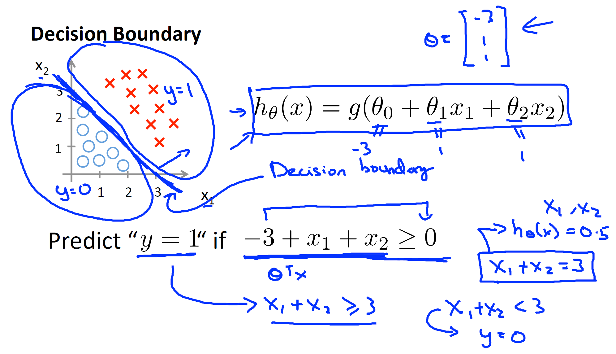
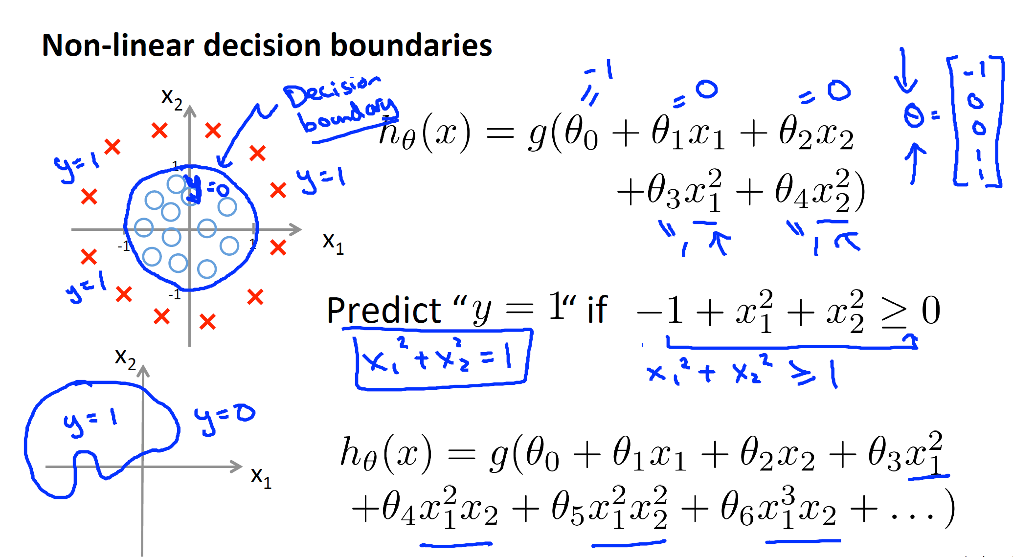
Machine Learning by Standford University on Coursera

6. Naive Bayes

6.1 What are the basic concepts/ What problem does it solve?

The Naive Bayes Algorithm is a classification method. It is primarily used for text classification, which involves high-dimensional training datasets, i.e spam filtration, sentimental analysis, and classifying news articles.

It learns the probability of an object with certain features belonging to a particular group in class, in short it is a probabilistic classifier.

6.2 What are the assumptions?

The Naive Bayes algorithm is called “naive” because it makes the assumption that the occurrence of a certain feature is independent of the occurrence of other features.

Bayes’ Theorem

$P(A \vert B)= \frac{P(B\vert A) P(A)}{P(B)}$ where $A$ and $B$ are events and $P(B)\neq 0$.

• $P(A\vert B)$ is a conditional probability: the likelihood of event $A$ occurring given that $B$ is true.

• $P(B\vert A)$ is a conditional probability: the likelihood of event $B$ occurring given that $A$ is true.

• $P(A)$ and $P(B)$ are the probabilities of observing $A$ and $B$ independently of each other, also known as the marginal probability.

Naive Bayes Theorem

In Naive Bayes Theorem,

• A:= proposition; B:= evidence

• $P(A)$:= prior probability of proposition, $P(B)$ prior probability of evidence

• $P(A\vert B)$:= posterior

• $P(B\vert A)$:= likelihood

$$Posterior= \frac{Likelihood \cdot Proposition \quad prior \quad probability}{Evidence \quad prior \quad probability}$$

6.3 What is the process of the algorithm?

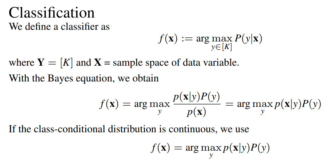
naive bayes classifiers - Columbia Statistics



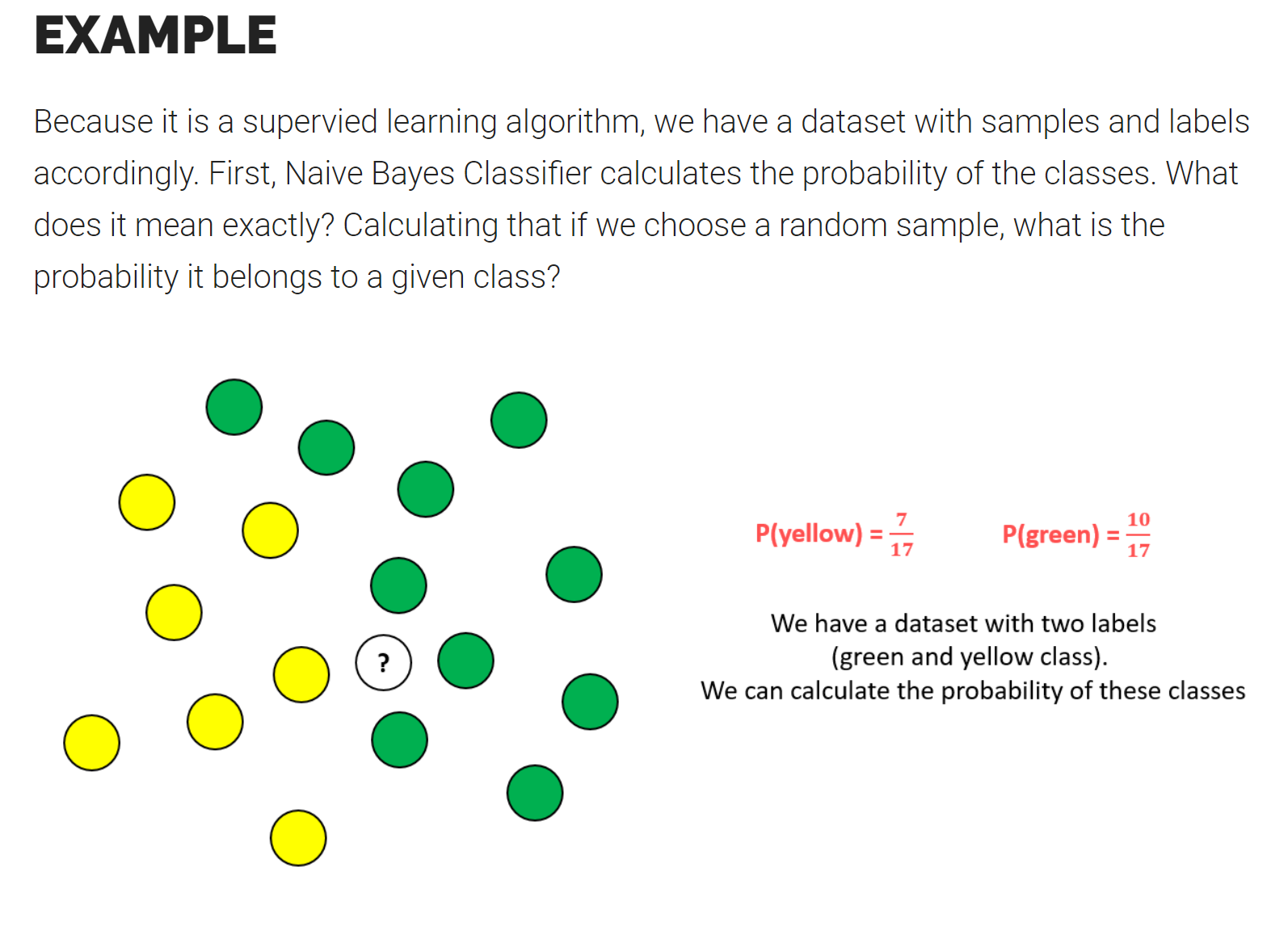
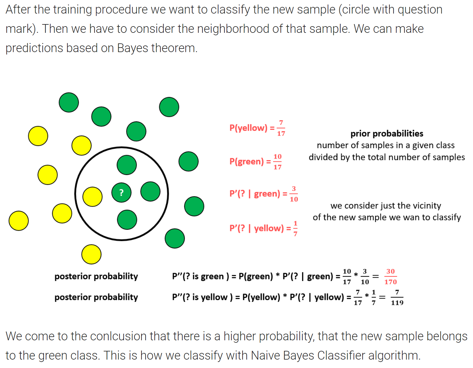
Naive Bayes Classifier Explained Step by Step

6.4 What is the cost function?

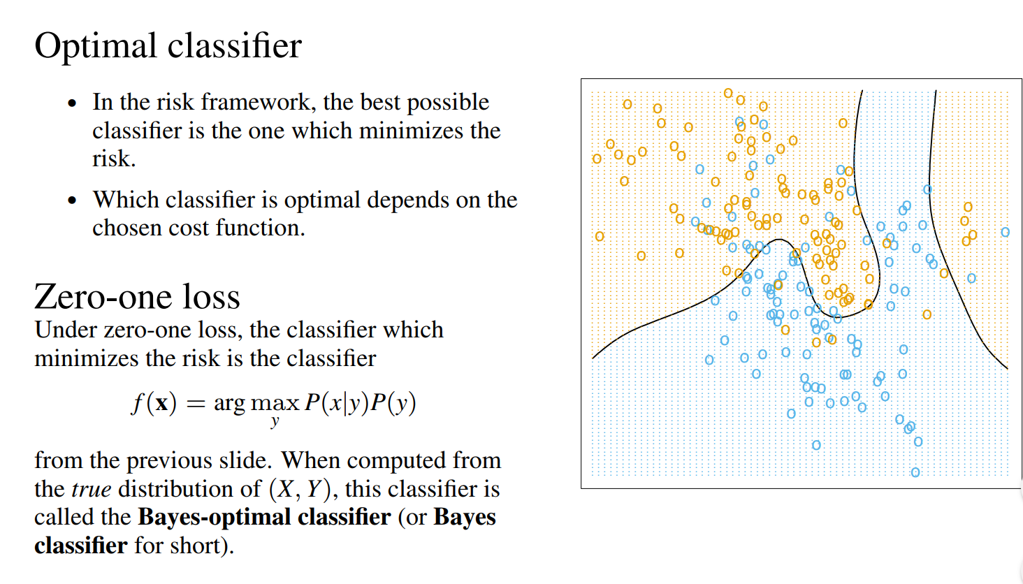
naive bayes classifiers - Columbia Statistics

6.6 What are the Advantages and Disadvantages? Advantages:

• It is easy and fast to predict class of test data set. It also perform well in multi class prediction.

• When assumption of independence holds, a Naive Bayes classifier performs better compare to other models like logistic regression and you need less training data.

• It perform well in case of categorical input variables compared to numerical variables, which is assumed normally distributed.

Disadvantages:

• If there is a category in the test dataset not observed in training data set, then model will assign a zero probability and cannot make a prediction. This is often known as “Zero Frequency”. To solve this, we can use the smoothing technique. One of the simplest smoothing techniques is called Laplace estimation.

• Naive Bayes is also known as a bad estimator, so the predicted probability are not to be taken too seriously.

• Naive Bayes is the assumption of independent predictors. In real life, it is almost impossible that we get a set of predictors which are completely independent.

6.7 Additions of Naive Bayes

6.7.1 Variations of Naive Bayes

• Gaussian: It is used in classification and it assumes that features follow a normal distribution.

• Multinomial: It is used for discrete counts.

• Bernoulli: The binomial model is useful if your feature vectors are binary (i.e. zeros and ones) .Like the multinomial model, this model is popular for document classification tasks, where binary term occurrence features are used rather than term frequencies.

6.7.2 Some real-world applications of Naive Bayes

• Real time Prediction: Naive Bayes is an eager learning classifier and it is sure fast. Thus, it could be used for making predictions in real time.

• Text classification/Spam Filtering/Sentiment Analysis: Naive Bayes classifiers mostly used in text classification (due to better result in multi class problems and independence rule) have higher success rate as compared to other algorithms. As a result, it is widely used in Spam filtering (identify spam e-mail) and Sentiment Analysis (in social media analysis, to identify positive and negative customer sentiments)

• Recommendation System: Naive Bayes Classifier and Collaborative Filtering together builds a Recommendation System that uses machine learning and data mining techniques to filter unseen information and predict whether a user would like a given resource or not

7. LDA (Linear Discriminant Analysis)

7.1 What are the basic concepts/ What problem does it solve?

LDA is an alternative approach to logistic regression, we model the distribution of the predictors $X$ separately in each of the response classes (i.e. given $Y$ ), and then use Bayes’ theorem to flip these around into estimates for $Pr(Y = k\vert X = x)$.

7.2 What are the assumptions?

• The observations in each class are drawn from a multivariate Gaussian distribution

• The distribution of all classes have the same class-specific mean vector and a covariance matrix

7.3 What is the process of the algorithm?

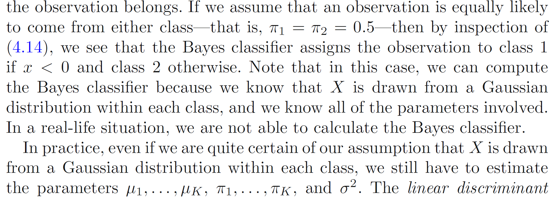
Recall the Bayes’ Theorem, $$P(Y=k \vert X=x)= \frac{\pi_k f_k(x)}{\sum_{l=1}^K \pi_l f_l(x)}$$

where, $K:$ number of classes, $K \ge 2$ and unordered

$\pi_k:$ the overall or prior probability that a randomly chosen observation comes from the $k^{th}$ class (this is the probability that a given observation is associated with the $k^{th}$ category of the response variable Y)

$fk(X) \equiv Pr(X = x \vert Y = k):$ the density function of $X$ for an observation that comes from the $k^{th}$ class.

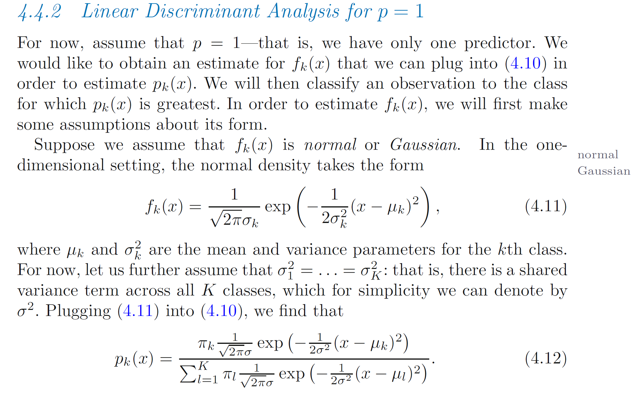
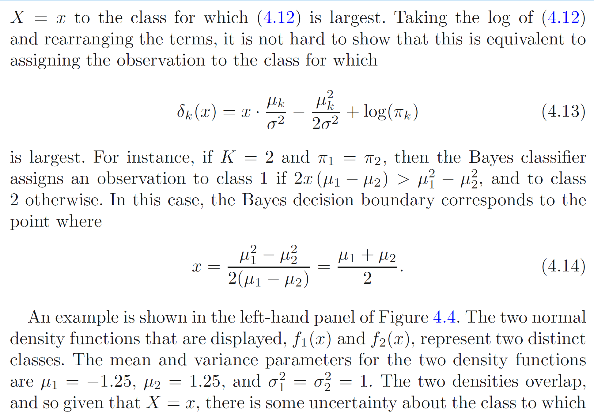
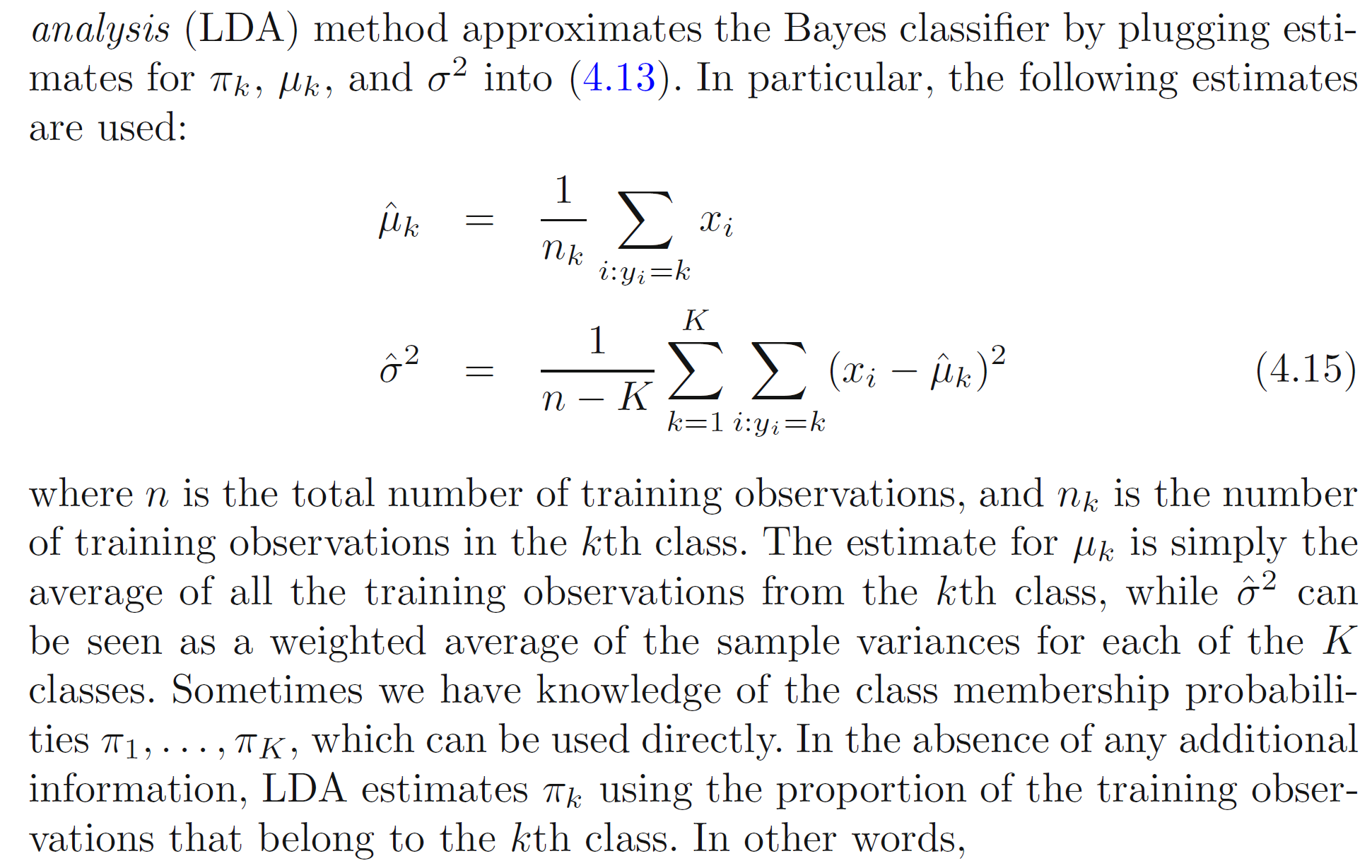
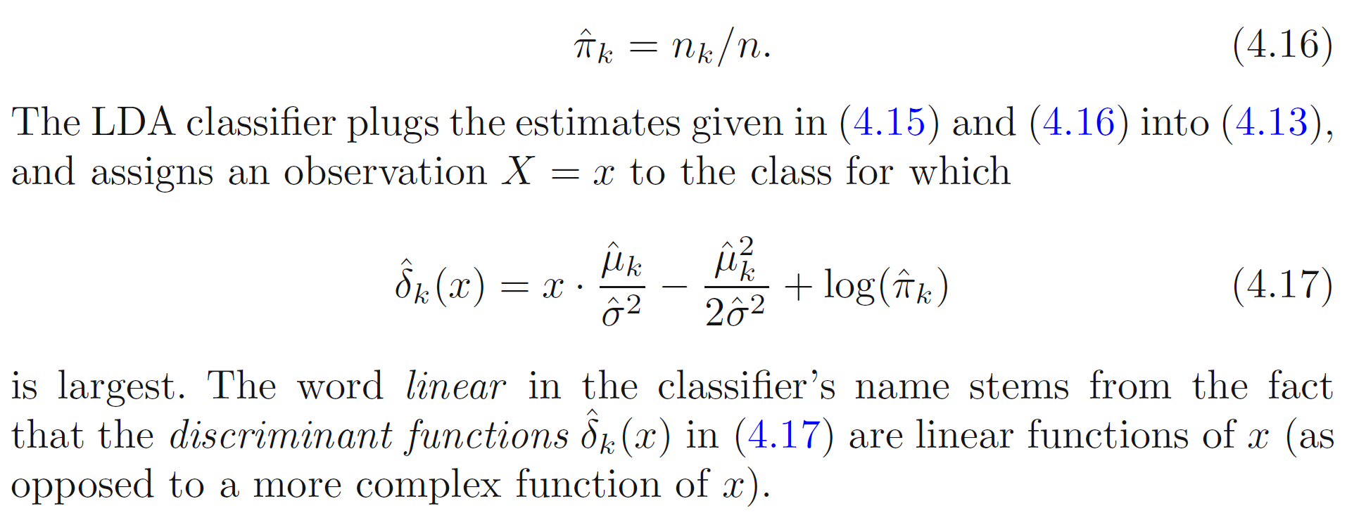
An Introduction to Statistical Learning with Applications in R-Springer

7.4 What is the cost function?

Same as naive bayes.

7.5 What are the advantages and disadvantages?

Advantages:

• When the classes are well-separated, the parameter estimates for the logistic regression model are surprisingly unstable. LDA does not suffer from this problem.

• If $n$ is small and the distribution of the predictors is approximately normal in each of the classes, LDA is again more stable than the logistic regression model.

• LDA is popular when we have more than two response classes.

Disadvantages:

• LDA only gives decision boundaries, sometimes cannot fit complex dataset, which means it will suffer from high bias.

8. QDA (Quadratic Discriminant Analysis)

8.1 What are the basic concepts/ What problem does it solve?

QDA provides another alternative approach. Like LDA, the QDA classifier results from assuming that the observations from each class are drawn from a Gaussian distribution, and plugging estimates for the parameters into Bayes’ theorem in order to perform prediction.

8.2 What are the assumptions?

• The observations in each class are drawn from a multivariate Gaussian distribution

• Each class has its own covariance matrix.

8.3 What is the process of the algorithm?

QDA assumes that an observation from the $k^{th}$ class is of the form $X \sim N(\mu_k, \Sigma_k)$, where $\Sigma_k$ is a covariance matrix for the $k^{th}$ class.

Under this assumption, the Bayes classifier assigns an observation $X = x$ to the class for which $$ \sigma_k(x) = -\frac{1}{2}(x-\mu_k)^T \Sigma_k^{-1} (x-\mu_k)- \frac{1}{2} log \vert \Sigma_k \vert+ log\pi_k $$ is largest.

So the QDA classifier involves plugging estimates for $\Sigma_k(x)$, $\mu_k$, and $\pi_k$, and then assigning an observation $X = x$ to the class for which this quantity is largest.

The quantity $x$ appears as a quadratic function in, this is where QDA gets its name.

8.4 What is the cost function?

Same as naive bayes.

8.5 What are the advantages and disadvantages? (LDA V.S QDA)

Advantages:

• QDA is recommended if the training set is very large if the assumption of a common covariance matrix for the $K$ classes is clearly untenable.

Disadvantages:

• QDA estimates a separate covariance matrix for each class, for a total of $Kp(p+1)/2$ parameters. So, if we have 50 predictors, then there are some multiple of 1225, which is a lot of parameters. But in LDA model, there are $Kp$ linear coefficients to estimate.

• LDA is a much less flexible classifier than QDA, and so has substantially lower variance, potentially lead to improved prediction performance.

• LDA tends to be a better bet than QDA if there are relatively few training observations and so reducing variance is crucial.